3. Problem statement

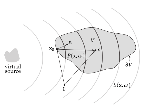
Fig. 3.1 Illustration of the geometry used to discuss the physical fundamentals of sound field synthesis and the single-layer potential.

The problem of sound field synthesis can be formulated after as follows. Assume a volume \(V \subset \mathbb{R}^n\) which is free of any sources and sinks, surrounded by a distribution of monopole sources on its surface \(\partial V\). The pressure \(P(\x,\w)\) at a point \(\x\in V\) is then given by the single-layer potential (compare p. 39 in [CK98])

(3.1)\[P(\x,\w) = \oint_{\partial V} D(\x_0,\w) G(\x-\x_0,\w) \d A(\x_0),\]

where \(G(\x-\x_0,\w)\) denotes the sound propagation of the source at location \(\x_0 \in \partial V\), and \(D(\x_0,\w)\) its weight, usually referred to as driving function. The sources on the surface are called secondary sources in sound field synthesis, analogue to the case of acoustical scattering problems. The single-layer potential can be derived from the Kirchhoff-Helmholtz integral [Wil99]. The challenge in sound field synthesis is to solve the integral with respect to \(D(\x_0,\w)\) for a desired sound field \(P = S\) in \(V\). It has unique solutions which [ZS13] explicitly showed for the spherical case and [Faz10] (Chap.4.3) for the planar case.

In the following the single-layer potential for different dimensions is discussed. An approach to formulate the desired sound field \(S\) is described and finally it is shown how to derive the driving function \(D\).