6. Sound Field Dimensionality

The single-layer potential (3.1) is valid for all \(V \subset {\mathbb{R}}^n\). Consequentially, for practical applications a two-dimensional (2D) as well as a three-dimensional (3D) synthesis is possible. Two-dimensional is not referring to a synthesis in a plane only, but describes a setup that is independent of one dimension. For example, an infinite cylinder is independent of the dimension along its axis. The same is true for secondary source distributions in 2D synthesis. They exhibit line source characteristics and are aligned in parallel to the independent dimension. Typical arrangements of such secondary sources are a circular or a linear setup.

The characteristics of the secondary sources limit the set of possible sources which can be synthesized. For example, when using a 2D secondary source setup it is not possible to synthesize the amplitude decay of a point source.

For a 3D synthesis the involved secondary sources depend on all dimensions and exhibit point source characteristics. In this scenario classical secondary sources setups would be a sphere or a plane.

6.1. 2.5D Synthesis

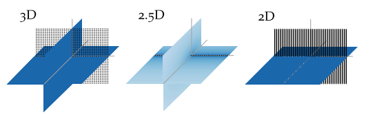
Fig. 6.1 Sound pressure in decibel for secondary source distributions with different dimensionality all driven by the same signals. The sound pressure is color coded, lighter color corresponds to lower pressure. In the 3D case a planar distribution of point sources is applied, in the 2.5D case a linear distribution of point sources, and in the 2D case a linear distribution of line sources.

In practice, the most common setups of secondary sources are 2D setups, employing cabinet loudspeakers. A cabinet loudspeaker does not show the characteristics of a line source, but of a point source. This dimensionality mismatch prevents perfect synthesis within the desired plane. The combination of a 2D secondary source setup with secondary sources that exhibit 3D characteristics has led to naming such configurations 2.5D synthesis [Sta97]. Such scenarios are associated with a wrong amplitude decay due to the inherent mismatch of secondary sources as is highlighted in Fig. 6.1. In general, the amplitude is only correct at a given reference point \(\xref\).

For a circular secondary source distribution with point source characteristic the 2.5D driving function can be derived by introducing expansion coefficients for the spherical case into the driving function (4.14). The equation is than solved for \(\theta = 0{^\circ}\) and \(r_\text{ref} = 0\). This results in a 2.5D driving function given after [Ahr12], eq. (3.49) as

(6.1)\[D_{\text{circular},\text{2.5D}}(\phi_0,\w) = \frac{1}{2\pi R_0} \sum_{m=-\infty}^\infty \frac{\breve{S}_{|m|}^m (\frac{\pi}{2},\phi_\text{s},r_\text{s},\w)}{\breve{G}_{|m|}^m (\frac{\pi}{2},0,\w)} \Phi_m(\phi_0).\]

For a linear secondary source distribution with point source characteristics the 2.5D driving function is derived by introducing the linear expansion coefficients for a monopole source (7.9) into the driving function (4.22) and solving the equation for \(y = y_\text{ref}\) and \(z = 0\). This results in a 2.5D driving function given after [Ahr12], eq. (3.77) as

(6.2)\[D_{\text{linear},\text{2.5D}}(x_0,\w) = \frac{1}{2\pi} \int_{-\infty}^\infty \frac{\breve{S}(k_x,y_\text{ref},0,\w)} {\breve{G}(k_x,y_\text{ref},0,\w)} \chi(k_x,x_0) \d k_x.\]

A driving function for the 2.5D situation in the context of WFS and arbitrary 2D geometries of the secondary source distribution can be achieved by applying the far-field approximation \(\Hankel{2}{0}{\zeta} \approx \sqrt{\frac{2\i}{\pi\zeta}} \e{-\i\zeta}\) for \(\zeta \gg 1\) to the 2D Green’s function [Wil99], eq. (4.23). Using this the following relationship between the 2D and 3D Green’s functions can be established.

(6.3)\[\begin{gathered} \underbrace{-\frac{\i}{4} \; \Hankel{2}{0}{\wc |\x-\x_0|}}_{G_\text{2D}(\x-\x_0,\w)} \approx \sqrt{2\pi\frac{c}{\i\w} |\x-\x_0|} \; \underbrace{ \frac{1}{4 \pi} \frac{\e{-\i\wc |\x-\x_0|}} {|\x-\x_0|}}_{G_\text{3D}(\x-\x_0,\w)}, \end{gathered}\]

where \(\Hankel{2}{0}{}\) denotes the Hankel function of second kind and zeroth order. Inserting this approximation into the single-layer potential for the 2D case results in

(6.4)\[P(\x,\w) = \oint_S \sqrt{2\pi\frac{c}{\i\w} |\x-\x_0|} \; D(\x_0,\w) G_\text{3D}(\x-\x0,\w) \d A(\x_0).\]

If the amplitude correction is further restricted to one reference point \(\xref\), the 2.5D driving function for WFS can be formulated as

(6.5)\[D_\text{2.5D}(\x_0,\w) = \underbrace{\sqrt{2\pi|\xref-\x_0|}}_{g_0} \sqrt{\frac{c}{\i\w}} \, D(\x_0,\w),\]

where \(g_0\) is independent of \(\x\).