9. Driving functions for WFS
In the following, the driving functions for WFS in the frequency and temporal domain for selected source models are presented. The temporal domain functions consist of a filtering of the source signal and a weighting and delaying of the individual secondary source signals. This property allows for a very efficient implementation of WFS driving functions in the temporal domain. It is one of the main advantages of WFS in comparison to most of the NFC-HOA, SDM solutions discussed above.
9.1. Plane Wave
nk = 0, -1, 0  # direction of plane wave
omega = 2 * np.pi * 1000  # frequency
xref = 0, 0, 0  # 2.5D reference point
x0, n0, a0 = sfs.array.circular(200, 1.5)
grid = sfs.util.xyz_grid([-1.75, 1.75], [-1.75, 1.75], 0, spacing=0.02)
d = sfs.mono.drivingfunction.wfs_25d_plane(omega, x0, n0, nk, xref)
a = sfs.mono.drivingfunction.source_selection_plane(n0, nk)
twin = sfs.tapering.tukey(a, .3)
p = sfs.mono.synthesized.generic(omega, x0, n0, d * twin * a0 , grid,
    source=sfs.mono.source.point)
normalization = 0.5
sfs.plot.soundfield(normalization * p, grid)
sfs.plot.secondarysource_2d(x0, n0, grid)
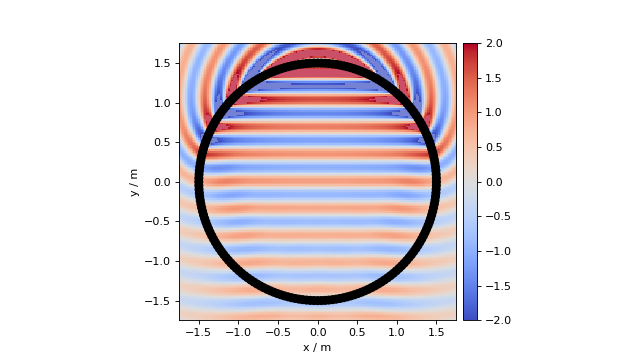
Fig. 9.1 Sound pressure for a monochromatic plane wave synthesized with 2.5D WFS (9.10). Parameters: \(\n_k = (0, -1, 0)\), \(\xref = (0, 0, 0)\), \(f = 1\) kHz.
By inserting the source model of a plane wave (7.1) into (5.2) and (6.5) it follows
Transferred to the temporal domain via an inverse Fourier transform (2.2), it follows
where
and
denote the so called pre-equalization filters in WFS.
The window function \(w(\x_0)\) for a plane wave as source model can be calculated after [SRA08] as
9.2. Point Source
xs = 0, 2.5, 0  # position of source
omega = 2 * np.pi * 1000  # frequency
xref = 0, 0, 0  # 2.5D reference point
x0, n0, a0 = sfs.array.circular(200, 1.5)
grid = sfs.util.xyz_grid([-1.75, 1.75], [-1.75, 1.75], 0, spacing=0.02)
d = sfs.mono.drivingfunction.wfs_25d_point(omega, x0, n0, xs, xref)
a = sfs.mono.drivingfunction.source_selection_point(n0, x0, xs)
twin = sfs.tapering.tukey(a, .3)
p = sfs.mono.synthesized.generic(omega, x0, n0, d * twin * a0 , grid,
    source=sfs.mono.source.point)
normalization = 1.3
sfs.plot.soundfield(normalization * p, grid)
sfs.plot.secondarysource_2d(x0, n0, grid)
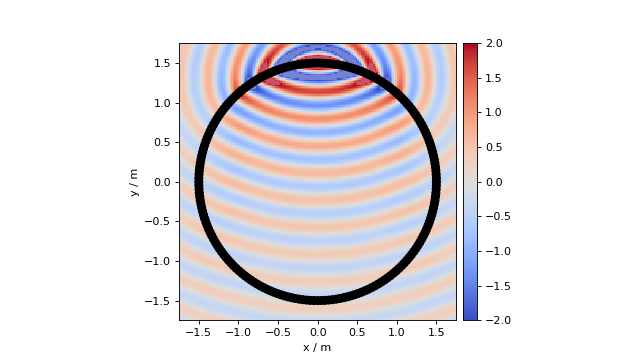
Fig. 9.2 Sound pressure for a monochromatic point source synthesized with 2.5D WFS (9.10). Parameters: \(\xs = (0, 2.5, 0)\) m, \(\xref = (0, 0, 0)\), \(f = 1\) kHz.
By inserting the source model for a point source (7.6) into (5.2) it follows
Under the assumption of \(\wc |\x_0-\xs| \gg 1\), (9.8) can be approximated by [Sch16], eq. (2.118)
It has the advantage that its temporal domain version could again be implemented as a simple weighting- and delaying-mechanism.
To reach at 2.5D for a point source, we will start in 3D and apply stationary phase approximations instead of directly using (6.5) – see discussion after [Sch16], (2.146). Under the assumption of \(\frac{\omega}{c} (|\x_0-\xs| + |\x-\x_0|) \gg 1\) it then follows [Sch16], eq. (2.137), [Sta97], eq. (3.10, 3.11)
whereby \(\xref\) is a reference point at which the synthesis is correct. A second stationary phase approximation can be applied to reach at [Sch16], eq. (2.131, 2.141), [Sta97], eq. (3.16, 3.17)
which is the traditional formulation of a point source in WFS as given by eq. (2.27) in [Ver97] [1]. Now \(d_\text{ref}\) is the distance of a line parallel to the secondary source distribution and \(d_\text{s}\) the shortest possible distance from the point source to the linear secondary source distribution.
The default WFS driving functions for a point source in the SFS Toolbox are (9.9) and (9.10). Transferring both to the temporal domain via an inverse Fourier transform (2.2) it follows
The window function \(w(\x_0)\) for a point source as source model can be calculated after [SRA08] as
9.3. Line Source
xs = 0, 2.5, 0  # position of source
omega = 2 * np.pi * 1000  # frequency
x0, n0, a0 = sfs.array.circular(200, 1.5)
grid = sfs.util.xyz_grid([-1.75, 1.75], [-1.75, 1.75], 0, spacing=0.02)
d = sfs.mono.drivingfunction.wfs_2d_line(omega, x0, n0, xs)
a = sfs.mono.drivingfunction.source_selection_line(n0, x0, xs)
twin = sfs.tapering.tukey(a, .3)
p = sfs.mono.synthesized.generic(omega, x0, n0, d * twin * a0 , grid,
    source=sfs.mono.source.point)
normalization = 7
sfs.plot.soundfield(normalization * p, grid)
sfs.plot.secondarysource_2d(x0, n0, grid)
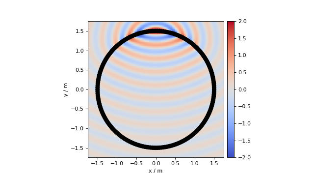
Fig. 9.3 Sound pressure for a monochromatic line source synthesized with 2D WFS (9.17). Parameters: \(\xs = (0, 2.5, 0)\) m, \(\xref = (0, 0, 0)\), \(f = 1\) kHz.
For a line source its orientation \(\n_\text{s}\) has an influence on the synthesized sound field as well. Let \(|\vec{v}|\) be the distance between \(\x_0\) and the line source with
where \(|\n_\text{s}| = 1\). For a 2D or 2.5D secondary source setup and a line source orientation perpendicular to the plane where the secondary sources are located this automatically simplifies to \(\vec{v} = \x_0 - \xs\).
By inserting the source model for a line source (7.12) into (5.2) and (6.5) and calculating the derivate of the Hankel function after http://dlmf.nist.gov/10.6.E6 it follows
Applying \(\Hankel{2}{1}{\zeta} \approx -\sqrt{\frac{2}{\pi\i}\zeta} \e{-\i\zeta}\) for \(z\gg1\) after [Wil99], eq. (4.23) and transferred to the temporal domain via an inverse Fourier transform (2.2) it follows
The window function \(w(\x_0)\) for a line source as source model can be calculated after [SRA08] as
9.4. Focused Source
xs = 0, 0.5, 0  # position of source
ns = 0, -1, 0  # direction of source
omega = 2 * np.pi * 1000  # frequency
xref = 0, 0, 0  # 2.5D reference point
x0, n0, a0 = sfs.array.circular(200, 1.5)
grid = sfs.util.xyz_grid([-1.75, 1.75], [-1.75, 1.75], 0, spacing=0.02)
d = sfs.mono.drivingfunction.wfs_25d_focused(omega, x0, n0, xs, xref)
a = sfs.mono.drivingfunction.source_selection_focused(ns, x0, xs)
twin = sfs.tapering.tukey(a, .3)
p = sfs.mono.synthesized.generic(omega, x0, n0, d * twin * a0 , grid,
    source=sfs.mono.source.point)
normalization = 1
sfs.plot.soundfield(normalization * p, grid)
sfs.plot.secondarysource_2d(x0, n0, grid)
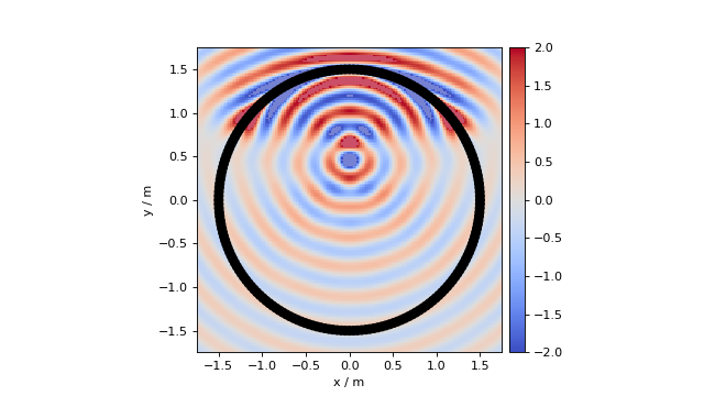
Fig. 9.4 Sound pressure for a monochromatic focused source synthesized with 2.5D WFS (9.23). Parameters: \(\xs = (0, 0.5, 0)\) m, \(\n_\text{s} = (0, -1, 0)\), \(\xref = (0, 0, 0)\), \(f = 1\) kHz.
As mentioned before, focused sources exhibit a field that converges in a focal point inside the audience area. After passing the focal point, the field becomes a diverging one as can be seen in Fig. 9.4. In order to choose the active secondary sources, especially for circular or spherical geometries, the focused source also needs a direction \(\n_\text{s}\).
The driving function for a focused source is given by the time-reversed versions of the driving function for a point source (9.12) and (9.13) as
The 2.5D driving functions are given by the time-reversed version of (9.13) for a reference point after [Ver97], eq. (A.14) as
and the time reversed version of (9.14) for a reference line, compare [Sta97], eq. (3.16)
where \(d_\text{ref}\) is the distance of a line parallel to the secondary source distribution and \(d_\text{s}\) the shortest possible distance from the focused source to the linear secondary source distribution.
Transferred to the temporal domain via an inverse Fourier transform (2.2) it follows
In this document a focused source always refers to the time-reversed version of a point source, but a focused line source can be defined in the same way starting from (9.17)
Transferred to the temporal domain via an inverse Fourier transform (2.2) it follows
The window function \(w(\x_0)\) for a focused source can be calculated as
| [1] | Whereby \(r\) corresponds to \(|\x_0-\xs|\) and \(\cos\varphi\) to \(\frac{\scalarprod{\x_0-\xs}{\n_{\x_0}}}{|\x_0-\xs|}\). |