8. Driving functions for NFC-HOA and SDM
In the following, driving functions for NFC-HOA and SDM are derived for spherical, circular, and linear secondary source distributions. Among the possible combinations of methods and secondary sources not all are meaningful. Hence, only the relevant ones will be presented. The same holds for the introduced source models of plane waves, point sources, line sources and focused sources. Ahrens and Spors [AS10] in addition have considered SDM driving functions for planar secondary source distributions.
For NFC-HOA, temporal-domain implementations for the 2.5D cases are available for a plane wave and a point source as source models. The derivation of the implementation is not explicitly shown here, but is described in [SKA11].
8.1. Plane Wave
nk = 0, -1, 0  # direction of plane wave
omega = 2 * np.pi * 1000  # frequency
R0 = 1.5  # radius of secondary sources
x0, n0, a0 = sfs.array.circular(200, R0)
grid = sfs.util.xyz_grid([-1.75, 1.75], [-1.75, 1.75], 0, spacing=0.02)
d = sfs.mono.drivingfunction.nfchoa_25d_plane(omega, x0, R0, nk)
p = sfs.mono.synthesized.generic(omega, x0, n0, d * a0 , grid,
    source=sfs.mono.source.point)
normalization = 0.05
sfs.plot.soundfield(normalization * p, grid)
sfs.plot.secondarysource_2d(x0, n0, grid)
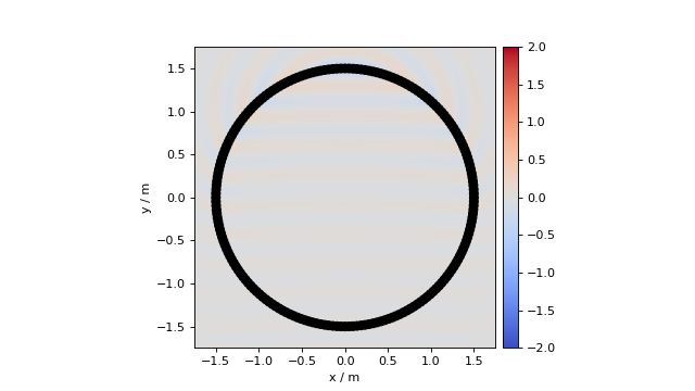
Fig. 8.1 Sound pressure for a monochromatic plane wave synthesized with 2.5D NFC-HOA (8.3). Parameters: \(\n_k = (0, -1, 0)\), \(\xref = (0, 0, 0)\), \(f = 1\) kHz.
For a spherical secondary source distribution with radius \(R_0\) the spherical expansion coefficients of a plane wave (7.3) and of the Green’s function for a point source (4.11) are inserted into (4.10) and yield [SS14], eq. (A3)
For a circular secondary source distribution with radius \(R_0\) the circular expansion coefficients of a plane wave (7.4) and of the Green’s function for a line source (4.15) are inserted into (4.14) and yield [AS09a], eq. (16)
For a circular secondary source distribution with radius \(R_0\) and point source as Green’s function the 2.5D driving function is given by inserting the spherical expansion coefficients for a plane wave (7.3) and a point source (7.8) into (6.1) as
For an infinite linear secondary source distribution located on the \(x\)-axis the 2.5D driving function is given by inserting the linear expansion coefficients for a point source as Green’s function (7.9) and a plane wave (7.5) into (6.2) and exploiting the fact that \((\wc )^2 - k_{x_\text{s}}\) is constant. Assuming \(0 \le |k_{x_\text{s}}| \le |\wc |\) this results in [AS10], eq. (17)
Transferred to the temporal domain this results in [AS10], eq. (18)
where \(\phi_k\) denotes the azimuth direction of the plane wave and
The advantage of this result is that it can be implemented by a simple weighting and delaying of the signal, plus one convolution with \(h(t)\). The same holds for the driving functions of WFS as presented in the next section.
8.2. Point Source
xs = 0, 2.5, 0  # position of source
omega = 2 * np.pi * 1000  # frequency
R0 = 1.5  # radius of secondary sources
x0, n0, a0 = sfs.array.circular(200, R0)
grid = sfs.util.xyz_grid([-1.75, 1.75], [-1.75, 1.75], 0, spacing=0.02)
d = sfs.mono.drivingfunction.nfchoa_25d_point(omega, x0, R0, xs)
p = sfs.mono.synthesized.generic(omega, x0, n0, d * a0 , grid,
    source=sfs.mono.source.point)
normalization = 20
sfs.plot.soundfield(normalization * p, grid)
sfs.plot.secondarysource_2d(x0, n0, grid)
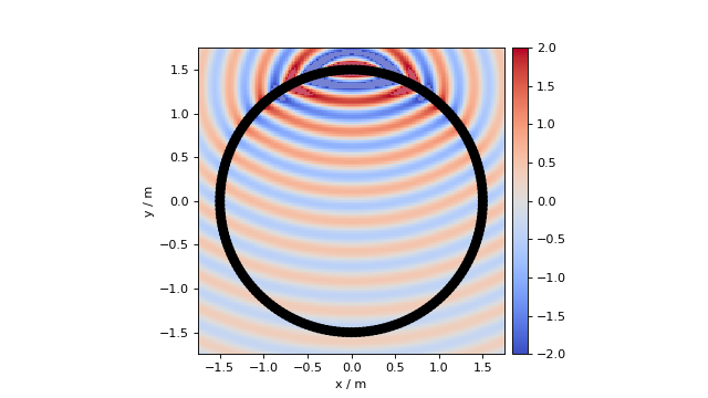
Fig. 8.2 Sound pressure for a monochromatic point source synthesized with 2.5D NFC-HOA (8.8). Parameters: \(\xs = (0, 2.5, 0)\) m, \(\xref = (0, 0, 0)\), \(f = 1\) kHz.
For a spherical secondary source distribution with radius \(R_0\) the spherical coefficients of a point source (7.8) and of the Green’s function (4.11) are inserted into (4.10) and yield [Ahr12], eq. (5.7) [1]
For a circular secondary source distribution with radius \(R_0\) and point source as secondary sources the 2.5D driving function is given by inserting the spherical coefficients (7.8) and (4.11) into (6.1). This results in [Ahr12], eq. (5.8)
For an infinite linear secondary source distribution located on the \(x\)-axis and point sources as secondary sources the 2.5D driving function for a point source is given by inserting the corresponding linear expansion coefficients (7.9) and (4.23) into (6.2). Assuming \(0 \le |k_x| < |\wc |\) this results in [Ahr12], eq. (4.53)
8.3. Line Source
For a spherical secondary source distribution with radius \(R_0\) the spherical coefficients of a line source (7.14) and of the Green’s function (4.11) are inserted into (4.10) and yield [HS15], eq. (20)
For a circular secondary source distribution with radius \(R_0\) and line sources as secondary sources the driving function is given by inserting the circular coefficients (7.15) and (4.15) into (4.14) as
For a circular secondary source distribution with radius \(R_0\) and point sources as secondary sources the 2.5D driving function is given by inserting the spherical coefficients (7.14) and (4.11) into (6.1) after [HS15], eq. (23) as
For an infinite linear secondary source distribution located on the \(x\)-axis and line sources as secondary sources the driving function is given by inserting the linear coefficients (7.16) and (4.23) into (4.22) as
8.4. Focused Source
Focused sources mimic point or line sources that are located inside the audience area. For the single-layer potential the assumption is that the audience area is free from sources and sinks. However, a focused source is neither of them. It represents a sound field that converges towards a focal point and diverges afterwards. This can be achieved by reversing the driving function of a point or line source in time which is known as time reversal focusing [YTF03].
Nonetheless, the single-layer potential should not be solved for focused sources without any approximation. In the near field of a source, evanescent waves appear for spatial frequencies \(k_x > |\wc |\) [Wil99], eq. (24). They decay exponentially with the distance from the source. An exact solution for a focused source is supposed to include these evanescent waves around the focal point. That is only possible by applying very large amplitudes to the secondary sources, compare Fig. 2a in [SA10]. Since the evanescent waves decay rapidly and are hence not influencing the perception, they can easily be omitted. For corresponding driving functions for focused sources without the evanescent part of the sound field see [SA10] for SDM and [AS09b] for NFC-HOA.
In the SFS Toolbox only focused sources in WFS are considered at the moment.
| [1] | Note the \(\frac{1}{2\pi}\) term is wrong in [Ahr12], eq. (3.21) and eq. (5.7) and omitted here, compare the errata and [SS14], eq. (24). |