Sound Field Synthesis
Sound field synthesis (SFS) includes all methods that try to generate a defined sound field in an extended area that is surrounded by loudspeakers. This page focuses on those methods that provide analytical solutions to the underlying mathematical problem, namely WFS, NFC-HOA, and the SDM.
The Toolboxes provide you with the implementation of the underlying mathematics. You can make numerical simulations of the resulting sound fields and can even create binaural simulations of the same sound fields. This enables you to listen to large loudspeaker arrays, even if you don’t have one in your laboratory or at home. In addition, you can easily plug-in your own algorithms in order to test or compare them.
The SFS Toolbox project is structured in the following three sub-projects.
- Discussion of Theory:
- http://sfstoolbox.org (current page)
- SFS Toolbox for Matlab/Octave:
- http://matlab.sfstoolbox.org
- SFS Toolbox for Python:
- http://python.sfstoolbox.org
Most of the figures in this page are directly created by the SFS Toolbox for Python. All of them display the corresponding code for creating them directly before the actual figure. In order to recreate them, you have to execute the following code first:
import numpy as np
import matplotlib.pyplot as plt
import sfs
plt.rcParams['figure.figsize'] = 8, 4.5  # inch
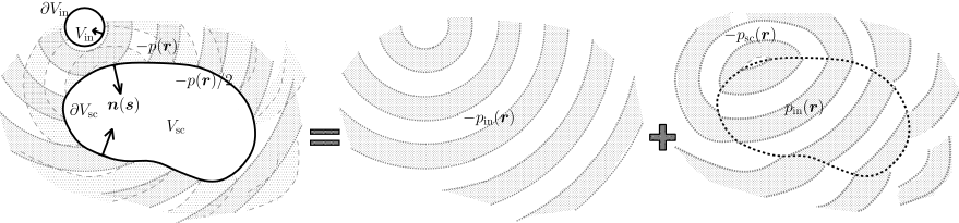
The image at the top of the page is extracted from [ZotterSpors2013]. The following presentation of the theory is based on Chap. 2 from [Wierstorf2014].
Mathematical Definitions
Coordinate system
Figure shows the coordinate system that is used in the following chapters. A vector \(\x\) can be described by its position \((x,y,z)\) in space or by its length, azimuth angle \(\phi \in [0,2\pi[\), and elevation \(\theta \in \left[-\frac{\pi}{2},\frac{\pi}{2}\right]\). The azimuth is measured counterclockwise and elevation is positive for positive \(z\)-values.
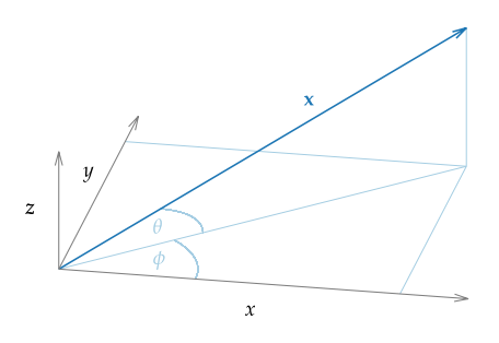
Fig. 1 Coordinate system used in this document. The vector \(x\) can also be described by its length, its azimuth angle \(\phi\), and its elevation \(\theta\).
Fourier transformation
Let \(s\) be an absolute integrable function, \(t,\w\) real numbers, then the temporal Fourier transform is defined after [Bracewell2000] as
In the same way the inverse temporal Fourier transform is defined as
Problem statement
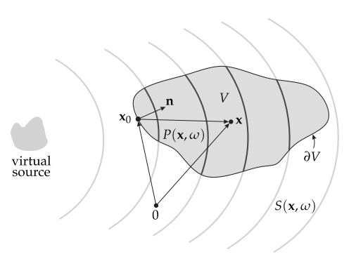
Fig. 2 Illustration of the geometry used to discuss the physical fundamentals of sound field synthesis and the single-layer potential.
The problem of sound field synthesis can be formulated after as follows. Assume a volume \(V \subset \mathbb{R}^n\) which is free of any sources and sinks, surrounded by a distribution of monopole sources on its surface \(\partial V\). The pressure \(P(\x,\w)\) at a point \(\x\in V\) is then given by the single-layer potential (compare p. 39 in [ColtonKress1998])
where \(G(\x-\x_0,\w)\) denotes the sound propagation of the source at location \(\x_0 \in \partial V\), and \(D(\x_0,\w)\) its weight, usually referred to as driving function. The sources on the surface are called secondary sources in sound field synthesis, analogue to the case of acoustical scattering problems. The single-layer potential can be derived from the Kirchhoff-Helmholtz integral [Williams1999]. The challenge in sound field synthesis is to solve the integral with respect to \(D(\x_0,\w)\) for a desired sound field \(P = S\) in \(V\). It has unique solutions which [ZotterSpors2013] explicitly showed for the spherical case and [Fazi2010] (Chap.4.3) for the planar case.
In the following the single-layer potential for different dimensions is discussed. An approach to formulate the desired sound field \(S\) is described and finally it is shown how to derive the driving function \(D\).
Solution for Special Geometries: NFC-HOA and SDM
The integral equation (3) states a Fredholm equation of first kind with a Green’s function as kernel. This type of equation can be solved in a straightforward manner for geometries that have a complete set of orthogonal basis functions. Then the involved functions are expanded into the basis functions \(\psi_n\) as [MorseFeshbach1981], p. (940)
where \(\tilde{G}_n, \tilde{D}_n, \tilde{S}_n\) denote the series expansion coefficients, \(n \in \mathbb{Z}\), and \(\langle\psi_n, \psi_{n'}\rangle = 0\,\) for \(n \ne n'\). If the underlying space is not compact the equations will involve an integration instead of a summation
where \(\d\mu\) is the measure in the underlying space. Introducing these equations into (3) one gets
This means that the Fredholm equation (3) states a convolution. For geometries where the required orthogonal basis functions exist, (10) follows directly via the convolution theorem [ArfkenWeber2005], eq. (1013). Due to the division of the desired sound field by the spectrum of the Green’s function this kind of approach has been named SDM [AhrensSpors2010]. For circular and spherical geometries the term NFC-HOA is more common due to the corresponding basis functions. “Near-field compensated” highlights the usage of point sources as secondary sources in contrast to Ambisonics and HOA that assume plane waves as secondary sources.
The challenge is to find a set of basis functions for a given geometry. In the following paragraphs three simple geometries and their widely known sets of basis functions will be discussed.
Spherical Geometries
The spherical harmonic functions constitute a basis for a spherical secondary source distribution in \({\mathbb{R}}^3\) and can be defined as [GumerovDuraiswami2004], eq. (12.153) [1]
where \(P_n^{|m|}\) are the associated Legendre functions. Note that this function may also be defined in a slightly different way, omitting the \((-1)^m\) factor, see for example [Williams1999], eq. (6.20).
The complex conjugate of \(Y_n^m\) is given by negating the degree \(m\) as
For a spherical secondary source distribution with a radius of \(R_0\) the sound field can be calculated by a convolution along the surface. The driving function is then given by a simple division as [Ahrens2012], eq. (3.21) [2]
where \(\breve{S}_n^m\) denote the spherical expansion coefficients of the source model, \(\theta_\text{s}\), \(\phi_\text{s}\), and \(r_\text{s}\) its directional dependency, and \(\breve{G}_n^0\) the spherical expansion coefficients of a secondary monopole source located at the north pole of the sphere \(\x_0 = (\frac{\pi}{2},0,R_0)\). For a point source this is given as [SchultzSpors2014], eq. (25)
where \(\hankel{2}{n}{}\) describes the spherical Hankel function of \(n\)-th order and second kind.
Circular Geometries
The following functions build a basis in \(\mathbb{R}^2\) for a circular secondary source distribution [Williams1999]
The complex conjugate of \(\Phi_m\) is given by negating the degree \(m\) as
For a circular secondary source distribution with a radius of \(R_0\) the driving function can be calculated by a convolution along the surface of the circle as explicitly shown by [AhrensSpors2009a] and is then given as
where \(\breve{S}_m\) denotes the circular expansion coefficients for the source model, \(\phi_\text{s}\), and \(r_\text{s}\) its directional dependency, and \(\breve{G}_m\) the circular expansion coefficients for a secondary monopole source. For a line source located at \(\x_0 = (0,R_0)\) this is given as
where \(\Hankel{2}{m}{}\) describes the Hankel function of \(m\)-th order and second kind.
Planar Geometries
The basis functions for a planar secondary source distribution located on the \(xz\)-plane in \(\mathbb{R}^3\) are given as
where \(k_x\), \(k_z\) are entries in the wave vector \(\k\) with \(k^2 = (\wc )^2\). The complex conjugate is given by negating \(k_x\) and \(k_z\) as
For an infinitely long secondary source distribution located on the \(xz\)-plane the driving function can be calculated by a two-dimensional convolution along the plane as [Ahrens2012], eq. (3.65)
where \(\breve{S}\) denotes the planar expansion coefficients for the source model, \(y_\text{s}\) its positional dependency, and \(\breve{G}\) the planar expansion coefficients of a secondary point source with [SchultzSpors2014], eq. (49)
for \((\wc )^2 > (k_x^2+k_z^2)\).
For the planar and the following linear geometries the Fredholm equation is solved for a non compact space \(V\), which leads to an infinite and non-denumerable number of basis functions as opposed to the denumerable case for compact spaces [SchultzSpors2014].
Linear Geometries
The basis functions for a linear secondary source distribution located on the \(x\)-axis are given as
The complex conjugate is given by negating \(k_x\) as
For an infinitely long secondary source distribution located on the \(x\)-axis the driving function for \({\mathbb{R}}^2\) can be calculated by a convolution along this axis as [Ahrens2012], eq. (3.73)
where \(\breve{S}\) denotes the linear expansion coefficients for the source model, \(y_\text{s}\), \(z_\text{s}\) its positional dependency, and \(\breve{G}\) the linear expansion coefficients of a secondary line source with
for \(0<|k_x|<|\wc |\,\).
High Frequency Approximation: WFS
The single-layer potential (3) satisfies the homogeneous Helmholtz equation both in the interior and exterior regions \(V\) and \(V^* {\mathrel{\!\mathop:}=}{\mathbb{R}}^n \setminus (V \cup \partial V)\,\). If \(D(\x_0,\w)\) is continuous, the pressure \(P(\x,\w)\) is continuous when approaching the surface \(\partial V\) from the inside and outside. Due to the presence of the secondary sources at the surface \(\partial V\), the gradient of \(P(\x,\w)\) is discontinuous when approaching the surface. The strength of the secondary sources is then given by the differences of the gradients approaching \(\partial V\) from both sides as [FaziNelson2013]
where \(\partial_\n{\mathrel{\mathop:}=}\scalarprod{\nabla}{\n}\) is the directional gradient in direction \(\n\) – see Fig. 2. Due to the symmetry of the problem the solution for an infinite planar boundary \(\partial V\) is given as
where the pressure in the outside region is the mirrored interior pressure given by the source model \(S(\x,\w)\) for \(\x\in V\). The integral equation resulting from introducing (28) into (3) for a planar boundary \(\partial V\) is known as Rayleigh’s first integral equation. This solution is identical to the explicit solution for planar geometries (21) in \({\mathbb{R}}^3\) and for linear geometries (25) in \({\mathbb{R}}^2\).
A solution of (27) for arbitrary boundaries can be found by applying the Kirchhoff or physical optics approximation [ColtonKress1983], p. 53–54. In acoustics this is also known as determining the visible elements for the high frequency boundary element method [Herrin2003]. Here, it is assumed that a bent surface can be approximated by a set of small planar surfaces for which (28) holds locally. In general, this will be the case if the wave length is much smaller than the size of a planar surface patch and the position of the listener is far away from the secondary sources. [3] Additionally, only one part of the surface is active: the area that is illuminated from the incident field of the source model.
The outlined approximation can be formulated by introducing a window function \(w(\x_0)\) for the selection of the active secondary sources into (28) as
In the SFS Toolbox we assume convex secondary source distributions, which allows to formulate the window function by a scalar product with the normal vector of the secondary source distribution. In general, also non-convex secondary source distributions can be used with WFS – compare the appendix in [LaxFeshbach1947] and [4].
One of the advantages of the applied approximation is that due to its local character the solution of the driving function (28) does not depend on the geometry of the secondary sources. This dependency applies to the direct solutions presented in Solution for Special Geometries: NFC-HOA and SDM.
Sound Field Dimensionality
The single-layer potential (3) is valid for all \(V \subset {\mathbb{R}}^n\). Consequentially, for practical applications a two-dimensional (2D) as well as a three-dimensional (3D) synthesis is possible. Two-dimensional is not referring to a synthesis in a plane only, but describes a setup that is independent of one dimension. For example, an infinite cylinder is independent of the dimension along its axis. The same is true for secondary source distributions in 2D synthesis. They exhibit line source characteristics and are aligned in parallel to the independent dimension. Typical arrangements of such secondary sources are a circular or a linear setup.
The characteristics of the secondary sources limit the set of possible sources which can be synthesized. For example, when using a 2D secondary source setup it is not possible to synthesize the amplitude decay of a point source.
For a 3D synthesis the involved secondary sources depend on all dimensions and exhibit point source characteristics. In this scenario classical secondary sources setups would be a sphere or a plane.
2.5D Synthesis
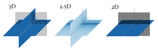
Fig. 3 Sound pressure in decibel for secondary source distributions with different dimensionality all driven by the same signals. The sound pressure is color coded, lighter color corresponds to lower pressure. In the 3D case a planar distribution of point sources is applied, in the 2.5D case a linear distribution of point sources, and in the 2D case a linear distribution of line sources.
In practice, the most common setups of secondary sources are 2D setups, employing cabinet loudspeakers. A cabinet loudspeaker does not show the characteristics of a line source, but of a point source. This dimensionality mismatch prevents perfect synthesis within the desired plane. The combination of a 2D secondary source setup with secondary sources that exhibit 3D characteristics has led to naming such configurations 2.5D synthesis [Start1997]. Such scenarios are associated with a wrong amplitude decay due to the inherent mismatch of secondary sources as is highlighted in Fig. 3. In general, the amplitude is only correct at a given reference point \(\xref\).
For a circular secondary source distribution with point source characteristic the 2.5D driving function can be derived by introducing expansion coefficients for the spherical case into the driving function (17). The equation is than solved for \(\theta = 0{^\circ}\) and \(r_\text{ref} = 0\). This results in a 2.5D driving function given as [Ahrens2012], eq. (3.49)
For a linear secondary source distribution with point source characteristics the 2.5D driving function is derived by introducing the linear expansion coefficients for a monopole source (43) into the driving function (25) and solving the equation for \(y = y_\text{ref}\) and \(z = 0\). This results in a 2.5D driving function given as [Ahrens2012], eq. (3.77)
A driving function for the 2.5D situation in the context of WFS and arbitrary 2D geometries of the secondary source distribution can be achieved by applying the far-field approximation \(\Hankel{2}{0}{\zeta} \approx \sqrt{\frac{2\i}{\pi\zeta}} \e{-\i\zeta}\) for \(\zeta \gg 1\) to the 2D Green’s function [Williams1999], eq. (4.23). Using this the following relationship between the 2D and 3D Green’s functions can be established.
where \(\Hankel{2}{0}{}\) denotes the Hankel function of second kind and zeroth order. Inserting this approximation into the single-layer potential for the 2D case results in
If the amplitude correction is further restricted to one reference point \(\xref\), 2.5D the driving function for WFS can be formulated as
where \(g_0\) is independent of \(\x\).
Model-Based Rendering
Knowing the pressure field of the desired source \(S(\x,\w)\) is required in order to derive the driving signal for the secondary source distribution. It can either be measured, i.e. recorded, or modeled. While the former is known as data-based rendering, the latter is known as model-based rendering. For data-based rendering, the problem of how to capture a complete sound field still has to be solved. [Avni2013] et al. discuss some influences of the recording limitations on the perception of the reproduced sound field. This document will consider only model-based rendering.
Frequently applied models in model-based rendering are plane waves, point sources, or sources with a prescribed complex directivity. In the following the models used within the SFS Toolbox are presented.
Plane Wave
nk = sfs.util.direction_vector(np.radians(45))  # direction of plane wave
xs = 0, 0, 0  # center of plane wave
omega = 2 * np.pi * 800  # frequency
grid = sfs.util.xyz_grid([-1.75, 1.75], [-1.75, 1.75], 0, spacing=0.02)
p = sfs.mono.source.plane(omega, xs, nk, grid)
sfs.plot.soundfield(p, grid);
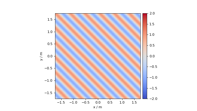
Fig. 4 Sound pressure for a monochromatic plane wave (36) going into the direction \((1, 1, 0)\). Parameters: \(f = 800\) Hz.
The source model for a plane wave is given as [Williams1999], eq. (2.24) [5]
where \(A(\w)\) denotes the frequency spectrum of the source and \(\n_k\) a unit vector pointing into the direction of the plane wave.
Transformed in the temporal domain this becomes
where \(a(t)\) is the Fourier transformation of the frequency spectrum \(A(\w)\).
The expansion coefficients for spherical basis functions are given as [Ahrens2012], eq. (2.38)
where \((\phi_k,\theta_k)\) is the radiating direction of the plane wave.
In a similar manner the expansion coefficients for circular basis functions are given as
The expansion coefficients for linear basis functions are given as after [Ahrens2012], eq. (C.5)
where \((k_{x,\text{s}},k_{y,\text{s}})\) points into the radiating direction of the plane wave.
Point Source
xs = 0, 0, 0  # position of source
omega = 2 * np.pi * 800  # frequency
grid = sfs.util.xyz_grid([-1.75, 1.75], [-1.75, 1.75], 0, spacing=0.02)
p = sfs.mono.source.point(omega, xs, [], grid)
normalization = 4 * np.pi
sfs.plot.soundfield(normalization * p, grid);
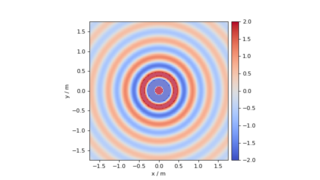
Fig. 5 Sound pressure for a monochromatic point source (41) placed at \((0, 0, 0)\). Parameters: \(f = 800\) Hz.
The source model for a point source is given by the three dimensional Green’s function as [Williams1999], eq. (6.73)
where \(\xs\) describes the position of the point source.
Transformed to the temporal domain this becomes
The expansion coefficients for spherical basis functions are given as [Ahrens2012], eq. (2.37)
where \((\phi_\text{s},\theta_\text{s},r_\text{s})\) describes the position of the point source.
The expansion coefficients for linear basis functions are given as [Ahrens2012], eq. (C.10)
for \(|k_x|<|\wc |\) and with \((x_\text{s},y_\text{s})\) describing the position of the point source.
Dipole Point Source
xs = 0, 0, 0  # position of source
ns = sfs.util.direction_vector(0)  # direction of source
omega = 2 * np.pi * 800  # frequency
grid = sfs.util.xyz_grid([-1.75, 1.75], [-1.75, 1.75], 0, spacing=0.02)
p = sfs.mono.source.point_dipole(omega, xs, ns, grid)
sfs.plot.soundfield(p, grid);
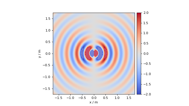
Fig. 6 Sound pressure for a monochromatic dipole point source (45) placed at \((0, 0, 0)\) and pointing towards \((1, 0, 0)\). Parameters: \(f = 800\) Hz.
The source model for a three dimensional dipole source is given by the directional derivative of the three dimensional Green’s function with respect to \({\n_\text{s}}\) defining the orientation of the dipole source.
Transformed to the temporal domain this becomes
Line Source
xs = 0, 0, 0  # position of source
omega = 2 * np.pi * 800  # frequency
grid = sfs.util.xyz_grid([-1.75, 1.75], [-1.75, 1.75], 0, spacing=0.02)
p = sfs.mono.source.line(omega, xs, None, grid)
normalization = np.sqrt(8 * np.pi * omega / sfs.defs.c) * np.exp(1j * np.pi / 4)
sfs.plot.soundfield(normalization * p, grid);
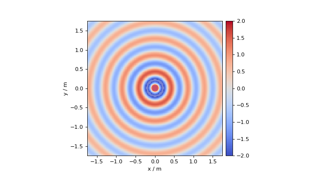
Fig. 7 Sound pressure for a monochromatic line source (47) placed at \((0, 0, 0)\). Parameters: \(f = 800\) Hz.
The source model for a line source is given by the two dimensional Green’s function as [Williams1999], eq. (8.47)
Applying the large argument approximation of the Hankel function [Williams1999], eq. (4.23) and transformed to the temporal domain this becomes
The expansion coefficients for spherical basis functions are given as [Hahn2015], eq. (15)
The expansion coefficients for circular basis functions are given as
The expansion coefficients for linear basis functions are given as
Driving functions for NFC-HOA and SDM
In the following, driving functions for NFC-HOA and SDM are derived for spherical, circular, and linear secondary source distributions. Among the possible combinations of methods and secondary sources not all are meaningful. Hence, only the relevant ones will be presented. The same holds for the introduced source models of plane waves, point sources, line sources and focused sources. [AhrensSpors2010] in addition have considered SDM driving functions for planar secondary source distributions.
For NFC-HOA, temporal-domain implementations for the 2.5D cases are available for a plane wave and a point source as source models. The derivation of the implementation is not explicitly shown here, but is described in [Spors2011].
Plane Wave
nk = 0, -1, 0  # direction of plane wave
omega = 2 * np.pi * 1000  # frequency
R0 = 1.5  # radius of secondary sources
x0, n0, a0 = sfs.array.circular(200, R0)
grid = sfs.util.xyz_grid([-1.75, 1.75], [-1.75, 1.75], 0, spacing=0.02)
d = sfs.mono.drivingfunction.nfchoa_25d_plane(omega, x0, R0, nk)
p = sfs.mono.synthesized.generic(omega, x0, n0, d * a0 , grid,
    source=sfs.mono.source.point)
normalization = 0.05
sfs.plot.soundfield(normalization * p, grid);
sfs.plot.secondarysource_2d(x0, n0, grid)
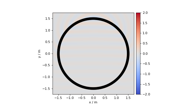
Fig. 8 Sound pressure for a monochromatic plane wave synthesized with 2.5D NFC-HOA (53). Parameters: \(\n_k = (0, -1, 0)\), \(\xref = (0, 0, 0)\), \(f = 1\) kHz.
For a spherical secondary source distribution with radius \(R_0\) the spherical expansion coefficients of a plane wave (37) and of the Green’s function for a point source (14) are inserted into (13) and yield [SchultzSpors2014], eq. (A3)
For a circular secondary source distribution with radius \(R_0\) the circular expansion coefficients of a plane wave (38) and of the Green’s function for a line source (18) are inserted into (17) and yield [AhrensSpors2009a], eq. (16)
For a circular secondary source distribution with radius \(R_0\) and point source as Green’s function the 2.5D driving function is given by inserting the spherical expansion coefficients for a plane wave (37) and a point source (42) into (30) as
For an infinite linear secondary source distribution located on the \(x\)-axis the 2.5D driving function is given by inserting the linear expansion coefficients for a point source as Green’s function (43) and a plane wave (39) into (31) and exploiting the fact that \((\wc )^2 - k_{x_\text{s}}\) is constant. Assuming \(0 \le |k_{x_\text{s}}| \le |\wc |\) this results in [AhrensSpors2010], eq. (17)
Transferred to the temporal domain this results in [AhrensSpors2010], eq. (18)
where \(\phi_k\) denotes the azimuth direction of the plane wave and
The advantage of this result is that it can be implemented by a simple weighting and delaying of the signal, plus one convolution with \(h(t)\). The same holds for the driving functions of WFS as presented in the next section.
Point Source
xs = 0, 2.5, 0  # position of source
omega = 2 * np.pi * 1000  # frequency
R0 = 1.5  # radius of secondary sources
x0, n0, a0 = sfs.array.circular(200, R0)
grid = sfs.util.xyz_grid([-1.75, 1.75], [-1.75, 1.75], 0, spacing=0.02)
d = sfs.mono.drivingfunction.nfchoa_25d_point(omega, x0, R0, xs)
p = sfs.mono.synthesized.generic(omega, x0, n0, d * a0 , grid,
    source=sfs.mono.source.point)
normalization = 20
sfs.plot.soundfield(normalization * p, grid);
sfs.plot.secondarysource_2d(x0, n0, grid)
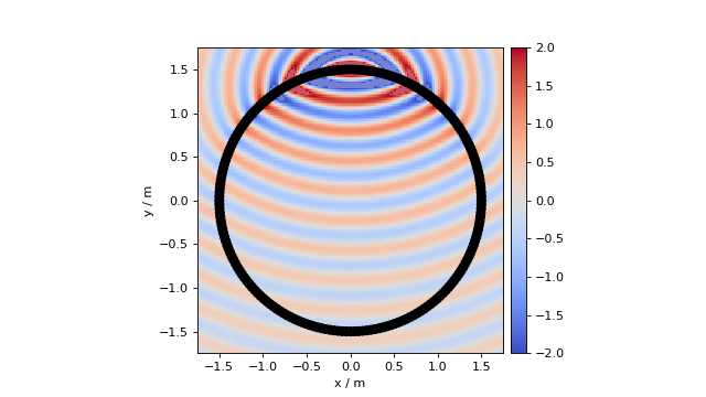
Fig. 9 Sound pressure for a monochromatic point source synthesized with 2.5D NFC-HOA (58). Parameters: \(\xs = (0, 2.5, 0)\) m, \(\xref = (0, 0, 0)\), \(f = 1\) kHz.
For a spherical secondary source distribution with radius \(R_0\) the spherical coefficients of a point source (42) and of the Green’s function (14) are inserted into (13) and yield [Ahrens2012], eq. (5.7) [2]
For a circular secondary source distribution with radius \(R_0\) and point source as secondary sources the 2.5D driving function is given by inserting the spherical coefficients (42) and (14) into (30). This results in [Ahrens2012], eq. (5.8)
For an infinite linear secondary source distribution located on the \(x\)-axis and point sources as secondary sources the 2.5D driving function for a point source is given by inserting the corresponding linear expansion coefficients (43) and (26) into (31). Assuming \(0 \le |k_x| < |\wc |\) this results in [Ahrens2012], eq. (4.53)
Line Source
For a spherical secondary source distribution with radius \(R_0\) the spherical coefficients of a line source (48) and of the Green’s function (14) are inserted into (13) and yield [Hahn2015], eq. (20)
For a circular secondary source distribution with radius \(R_0\) and line sources as secondary sources the driving function is given by inserting the circular coefficients (49) and (18) into (17) as
For a circular secondary source distribution with radius \(R_0\) and point sources as secondary sources the 2.5D driving function is given by inserting the spherical coefficients (48) and (14) into (30) as [Hahn2015], eq. (23)
For an infinite linear secondary source distribution located on the \(x\)-axis and line sources as secondary sources the driving function is given by inserting the linear coefficients (50) and (26) into (25) as
Focused Source
Focused sources mimic point or line sources that are located inside the audience area. For the single-layer potential the assumption is that the audience area is free from sources and sinks. However, a focused source is neither of them. It represents a sound field that converges towards a focal point and diverges afterwards. This can be achieved by reversing the driving function of a point or line source in time which is known as time reversal focusing [Yon2003].
Nonetheless, the single-layer potential should not be solved for focused sources without any approximation. In the near field of a source, evanescent waves appear for spatial frequencies \(k_x > |\wc |\) [Williams1999], eq. (24). They decay exponentially with the distance from the source. An exact solution for a focused source is supposed to include these evanescent waves around the focal point. That is only possible by applying very large amplitudes to the secondary sources, compare Fig. 2a in [SporsAhrens2010]. Since the evanescent waves decay rapidly and are hence not influencing the perception, they can easily be omitted. For corresponding driving functions for focused sources without the evanescent part of the sound field see [SporsAhrens2010] for SDM and [AhrensSpors2009b] for NFC-HOA.
In the SFS Toolbox only focused sources in WFS are considered at the moment.
Driving functions for WFS
In the following, the driving functions for WFS in the frequency and temporal domain for selected source models are presented. The temporal domain functions consist of a filtering of the source signal and a weighting and delaying of the individual secondary source signals. This property allows for a very efficient implementation of WFS driving functions in the temporal domain. It is one of the main advantages of WFS in comparison to most of the NFC-HOA, SDM solutions discussed above.
Plane Wave
nk = 0, -1, 0  # direction of plane wave
omega = 2 * np.pi * 1000  # frequency
xref = 0, 0, 0  # 2.5D reference point
x0, n0, a0 = sfs.array.circular(200, 1.5)
grid = sfs.util.xyz_grid([-1.75, 1.75], [-1.75, 1.75], 0, spacing=0.02)
d = sfs.mono.drivingfunction.wfs_25d_plane(omega, x0, n0, nk, xref)
a = sfs.mono.drivingfunction.source_selection_plane(n0, nk)
twin = sfs.tapering.tukey(a,.3)
p = sfs.mono.synthesized.generic(omega, x0, n0, d * twin * a0 , grid,
    source=sfs.mono.source.point)
normalization = 0.5
sfs.plot.soundfield(normalization * p, grid);
sfs.plot.secondarysource_2d(x0, n0, grid)
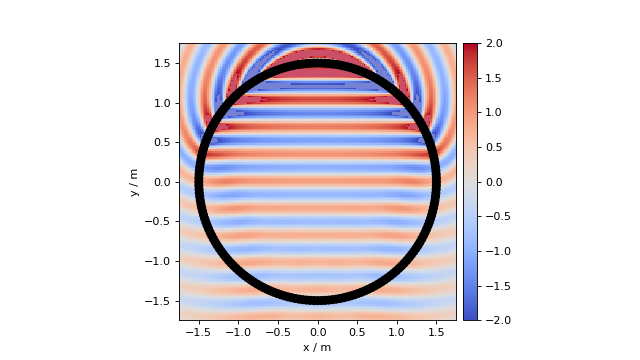
Fig. 10 Sound pressure for a monochromatic plane wave synthesized with 2.5D WFS (76). Parameters: \(\n_k = (0, -1, 0)\), \(\xref = (0, 0, 0)\), \(f = 1\) kHz.
By inserting the source model of a plane wave (36) into (28) and (34) it follows
Transferred to the temporal domain via an inverse Fourier transform (2), it follows
where
and
denote the so called pre-equalization filters in WFS.
The window function \(w(\x_0)\) for a plane wave as source model can be calculated after [Spors2008]
Point Source
xs = 0, 2.5, 0  # position of source
omega = 2 * np.pi * 1000  # frequency
xref = 0, 0, 0  # 2.5D reference point
x0, n0, a0 = sfs.array.circular(200, 1.5)
grid = sfs.util.xyz_grid([-1.75, 1.75], [-1.75, 1.75], 0, spacing=0.02)
d = sfs.mono.drivingfunction.wfs_25d_point(omega, x0, n0, xs, xref)
a = sfs.mono.drivingfunction.source_selection_point(n0, x0, xs)
twin = sfs.tapering.tukey(a,.3)
p = sfs.mono.synthesized.generic(omega, x0, n0, d * twin * a0 , grid,
    source=sfs.mono.source.point)
normalization = 1.3
sfs.plot.soundfield(normalization * p, grid);
sfs.plot.secondarysource_2d(x0, n0, grid)
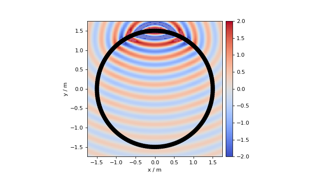
Fig. 11 Sound pressure for a monochromatic point source synthesized with 2.5D WFS (76). Parameters: \(\xs = (0, 2.5, 0)\) m, \(\xref = (0, 0, 0)\), \(f = 1\) kHz.
By inserting the source model for a point source (41) into (28) it follows
Under the assumption of \(\wc |\x_0-\xs| \gg 1\), (71) can be approximated by [Schultz2016], eq. (2.118)
It has the advantage that its temporal domain version could again be implemented as a simple weighting- and delaying-mechanism.
To reach at 2.5D for a point source, we will start in 3D and apply stationary phase approximations instead of directly using (34) – see discussion after [Schultz2016], (2.146). Under the assumption of \(\frac{\omega}{c} (|\x_0-\xs| + |\x-\x_0|) \gg 1\) it then follows [Schultz2016], eq. (2.137), [Start1997], eq. (3.10, 3.11)
whereby \(\xref\) is a reference point at which the synthesis is correct. A second stationary phase approximation can be applied to reach at [Schultz2016], eq. (2.131, 2.141), [Start1997], eq. (3.16, 3.17)
which is the traditional formulation of a point source in WFS as given by eq. (2.27) in [Verheijen1997] [6]. Now \(d_\text{ref}\) is the distance of a line parallel to the secondary source distribution and \(d_\text{s}\) the shortest possible distance from the point source to the linear secondary source distribution.
The default WFS driving functions for a point source in the SFS Toolbox are (75) and (76). Transferring both to the temporal domain via an inverse Fourier transform (2) it follows
The window function \(w(\x_0)\) for a point source as source model can be calculated after [Spors2008] as
Line Source
xs = 0, 2.5, 0  # position of source
omega = 2 * np.pi * 1000  # frequency
x0, n0, a0 = sfs.array.circular(200, 1.5)
grid = sfs.util.xyz_grid([-1.75, 1.75], [-1.75, 1.75], 0, spacing=0.02)
d = sfs.mono.drivingfunction.wfs_2d_line(omega, x0, n0, xs)
a = sfs.mono.drivingfunction.source_selection_line(n0, x0, xs)
twin = sfs.tapering.tukey(a,.3)
p = sfs.mono.synthesized.generic(omega, x0, n0, d * twin * a0 , grid,
    source=sfs.mono.source.point)
normalization = 7
sfs.plot.soundfield(normalization * p, grid);
sfs.plot.secondarysource_2d(x0, n0, grid)
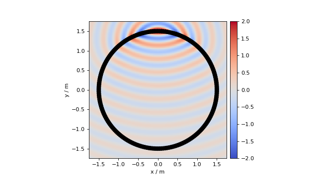
Fig. 12 Sound pressure for a monochromatic line source synthesized with 2D WFS (82). Parameters: \(\xs = (0, 2.5, 0)\) m, \(\xref = (0, 0, 0)\), \(f = 1\) kHz.
For a line source its orientation \(\n_\text{s}\) has an influence on the synthesized sound field as well. Let \(|\vec{v}|\) be the distance between \(\x_0\) and the line source with
where \(|\n_\text{s}| = 1\). For a 2D or 2.5D secondary source setup and a line source orientation perpendicular to the plane where the secondary sources are located this automatically simplifies to \(\vec{v} = \x_0 - \xs\).
By inserting the source model for a line source (47) into (28) and (34) and calculating the derivate of the Hankel function after eq. (9.1.20) in [AbramowitzStegun1972] it follows
Applying \(\Hankel{2}{1}{\zeta} \approx -\sqrt{\frac{2}{\pi\i}\zeta} \e{-\i\zeta}\) for \(z\gg1\) after [Williams1999], eq. (4.23) and transferred to the temporal domain via an inverse Fourier transform (2) it follows
The window function \(w(\x_0)\) for a line source as source model can be calculated after [Spors2008] as
Focused Source
xs = 0, 0.5, 0  # position of source
ns = 0, -1, 0  # direction of source
omega = 2 * np.pi * 1000  # frequency
xref = 0, 0, 0  # 2.5D reference point
x0, n0, a0 = sfs.array.circular(200, 1.5)
grid = sfs.util.xyz_grid([-1.75, 1.75], [-1.75, 1.75], 0, spacing=0.02)
d = sfs.mono.drivingfunction.wfs_25d_focused(omega, x0, n0, xs, xref)
a = sfs.mono.drivingfunction.source_selection_focused(ns, x0, xs)
twin = sfs.tapering.tukey(a,.3)
p = sfs.mono.synthesized.generic(omega, x0, n0, d * twin * a0 , grid,
    source=sfs.mono.source.point)
normalization = 1
sfs.plot.soundfield(normalization * p, grid);
sfs.plot.secondarysource_2d(x0, n0, grid)
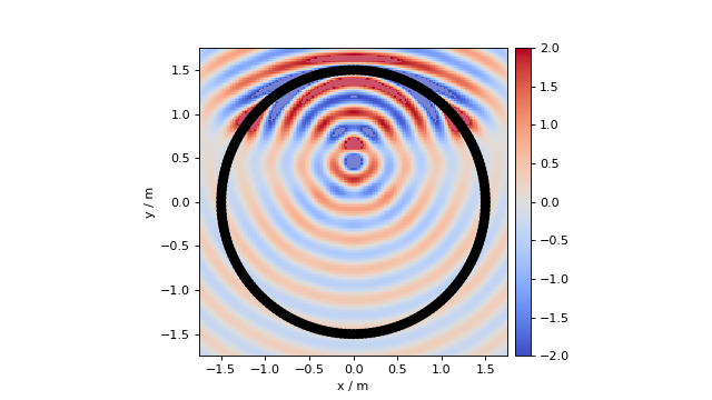
Fig. 13 Sound pressure for a monochromatic focused source synthesized with 2.5D WFS (89). Parameters: \(\xs = (0, 0.5, 0)\) m, \(\n_\text{s} = (0, -1, 0)\), \(\xref = (0, 0, 0)\), \(f = 1\) kHz.
As mentioned before, focused sources exhibit a field that converges in a focal point inside the audience area. After passing the focal point, the field becomes a diverging one as can be seen in Fig. 13. In order to choose the active secondary sources, especially for circular or spherical geometries, the focused source also needs a direction \(\n_\text{s}\).
The driving function for a focused source is given by the time-reversed versions of the driving function for a point source (75) and (76) as
The 2.5D driving functions are given by the time-reversed version of (76) for a reference point [Verheijen1997], eq. (A.14)
and the time reversed version of (77) for a reference line, compare [Start1997], eq. (3.16)
where \(d_\text{ref}\) is the distance of a line parallel to the secondary source distribution and \(d_\text{s}\) the shortest possible distance from the focused source to the linear secondary source distribution.
Transferred to the temporal domain via an inverse Fourier transform (2) it follows
In this document a focused source always refers to the time-reversed version of a point source, but a focused line source can be defined in the same way starting from (82)
Transferred to the temporal domain via an inverse Fourier transform (2) it follows
The window function \(w(\x_0)\) for a focused source can be calculated as
Driving functions for LSFS
The reproduction accuracy of WFS is limited due to practical aspects. For the audible frequency range the desired sound field can not be synthesized aliasing-free over an extended listening area, which is surrounded by a discrete ensemble of individually driven loudspeakers. However, it is suitable for certain applications to increase reproduction accuracy inside a smaller (local) listening region while stronger artifacts outside are permitted. This approach is termed LSFS in general.
The implemented Local Wave Field Synthesis method utilizes focused sources as a distribution of virtual loudspeakers which are placed more densely around the local listening area. These virtual loudspeakers can be driven by conventional SFS techniques, like e.g. WFS or NFC-HOA. The results are similar to band-limited NFC-HOA, with the difference that the form and position of the enhanced area can freely be chosen within the listening area.
The set of focused sources is treated as a virtual loudspeaker distribution and their positions \({\x_\text{fs}}\) are subsumed under \(\mathcal{X}_{\mathrm{fs}}\). Therefore, each focused source is driven individually by \(D_\text{l}({\x_\text{fs}}, \w)\), which in principle can be any driving function for real loudspeakers mentioned in previous sections. At the moment however, only WFS and NFC-HOA driving functions are supported. The resulting driving function for a loudspeaker located at \(\x_0\) reads
which is superposition of the driving function \(D_{\mathrm{fs}}(\x_0,{\x_\text{fs}},\w)\) reproducing a single focused source at \({\x_\text{fs}}\) weighted by \(D_\text{l}({\x_\text{fs}}, \w)\). Former is derived by replacing \(\xs\) with \({\x_\text{fs}}\) in the WFS driving functions and for focused sources. This yields
and
for the 2.5D case. For the temporal domain, inverse Fourier transform yields the driving signals
while \(d_{\mathrm{fs}}(\x_0,{\x_\text{fs}}, t)\) is derived analogously to from or . At the moment \(d_{\mathrm l}({\x_\text{fs}}, t)\) does only support driving functions from WFS.
Footnotes
| [1] | Note that \(\sin\theta\) is used here instead of \(\cos\theta\) due to the use of another coordinate system, compare Figure 2.1 from Gumerov and Duraiswami and Fig. 1. |
| [2] | (1, 2) Note the \(\frac{1}{2\pi}\) term is wrong in [Ahrens2012], eq. (3.21) and eq. (5.7) and omitted here, compare the errata and [SchultzSpors2014], eq. (24). |
| [3] | Compare the assumptions made before (15) in [SporsZotter2013], which lead to the derivation of the same window function in a more explicit way. |
| [4] | The solution mentioned by [LaxFeshbach1947] assumes that the listener is far away from the radiator and that the radiator is a physical source not a notional one as the secondary sources. In this case the selection criterion has to be chosen more carefully, incorporating the exact position of the listener and the virtual source. See also the related discussion. |
| [5] | Note that Williams defines the Fourier transform with transposed signs as \(F(\w) = \int f(t) \e{\i\w t}\). This leads also to changed signs in his definitions of the Green’s functions and field expansions. |
| [6] | Whereby \(r\) corresponds to \(|\x_0-\xs|\) and \(\cos\varphi\) to \(\frac{\scalarprod{\x_0-\xs}{\n_{\x_0}}}{|\x_0-\xs|}\). |
References
| [AbramowitzStegun1972] | Abramowitz, M. and Stegun, I. A., Handbook of Mathematical Functions. (National Bureau of Standards, Washington, 1972). |
| [Ahrens2012] | (1, 2, 3, 4, 5, 6, 7, 8, 9, 10, 11, 12, 13) Ahrens, J., Analytic Methods of Sound Field Synthesis. (Springer, New York, 2012). |
| [AhrensSpors2009a] | (1, 2) Ahrens, J. and Spors, S., “On the Secondary Source Type Mismatch in Wave Field Synthesis Employing Circular Distributions of Loudspeakers,” in 127th Conv. Audio Eng. Soc., New York, NY (2009), preprint 7952, url. |
| [AhrensSpors2009b] | Ahrens, J. and Spors, S., “Spatial encoding and decoding of focused virtual sound sources,” in 1st Ambisonics S., Graz, Austria (2009), url. |
| [AhrensSpors2010] | (1, 2, 3, 4) Ahrens, J. and Spors, S., “Sound Field Reproduction Using Planar and Linear Arrays of Loudspeakers,” IEEE Trans. Audio Speech Lang. Processing 18, 2038–2050 (2010), url. |
| [ArfkenWeber2005] | Arfken, G. B. and Weber, H. J., Mathematical Methods for Physicists. (Elsevier, Amsterdam, 2015). |
| [Avni2013] | Avni, A., Ahrens, J., Geier, M., Spors, S., Wierstorf, H., and Rafaely, B., “Spatial perception of sound fields recorded by spherical microphone arrays with varying spatial resolution,” J. Acoust. Soc. Am. 133, 2711–2721 (2013), url. |
| [Bracewell2000] | Bracewell, R. N., The Fourier Transform and its Applications. (McGraw Hill, Boston, 2000). |
| [ColtonKress1983] | Colton, D. and Kress, R., Integral Equation Methods in Scattering Theory. (Wiley, New York, 2000). |
| [ColtonKress1998] | Colton, D. and Kress, R., Inverse Acoustic and Electromagnetic Scattering Theory, (Springer, New York, 1998). |
| [Fazi2010] | Fazi, F. M., Sound Field Reproduction, Ph.D. dissertation, University of Southampton, Southampton, UK, 2010, url. |
| [FaziNelson2013] | Fazi, F. M. and Nelson, P. A., “Sound field reproduction as an equivalent acoustical scattering problem,” J. Acoust. Soc. Am. 134, 3721–3729 (2013), url. |
| [GumerovDuraiswami2004] | Gumerov, N. A. and Duraiswami, R., Fast Multipole Methods for the Helmholtz Equation in Three Dimensions. (Elsevier, Amsterdam, 2004). |
| [Hahn2015] | (1, 2, 3) Hahn, N. and Spors S., “Sound Field Synthesis of Virtual Cylindrical Waves Using Circular and Spherical Loudspeaker Arrays,” in 138th Conv. Audio Eng. Soc., Warsaw, Poland (2015), preprint 9324, url. |
| [Herrin2003] | Herrin, D. W., Martinus, F., Wu, T. W., and Seybert, A. F., “A New Look at the High Frequency Boundary Element and Rayleigh Integral Approximations,” SAE Technical Paper, doi:10.4271/2003-01-1451 (2003), url. |
| [LaxFeshbach1947] | (1, 2) Lax, M. and Feshbach, H., “On the Radiation Problem at High Frequencies,” J. Acoust. Soc. Am. 19, 682–690 (1947), url. |
| [MorseFeshbach1981] | Morse, P. M. and Feshbach, H., Methods of Theoretical Physics. (Feshbach Publishing, Minneapolis, 1981). |
| [SchultzSpors2014] | (1, 2, 3, 4, 5) Schultz, F. and Spors, S., “Comparing Approaches to the Spherical and Planar Single Layer Potentials for Interior Sound Field Synthesis,” Acta Acust. 100, 900–911 (2014), url. |
| [Schultz2016] | (1, 2, 3, 4) Schultz, F., Sound Field Synthesis for Line Source Array Applications in Large-Scale Sound Reinforcement, doctoral thesis, Universität Rostock, Rostock, Germany, 2016, url. |
| [SporsAhrens2010] | (1, 2) Spors, S. and Ahrens, J., “Reproduction of Focused Sources by the Spectral Division Method,” in 4th IEEE ISCCSP, Limassol, Cyprus (2010), doi:10.1109/ISCCSP.2010.5463335, url. |
| [SporsZotter2013] | Spors, S. and Zotter, F., “Spatial Sound Synthesis with Loudspeakers,” in Cutting Edge in Spatial Audio, EAA Winter School, Merano, Italy (2013), pp. 32–37, url. |
| [Spors2011] | Spors, S., Kuscher, V., and Ahrens, J., “Efficient realization of model-based rendering for 2.5-dimensional near-field compensated higher order Ambisonics,” in IEEE WASPAA, New Paltz, NY (2011), pp. 61–64, url. |
| [Spors2008] | (1, 2, 3) Spors, S., Rabenstein, R., and Ahrens, J., “The Theory of Wave Field Synthesis Revisited,” in 124th Conv. Audio Eng. Soc., Amsterdam, Netherlands (2008), preprint 7358, url. |
| [Start1997] | (1, 2, 3, 4) Start, E. W., Direct Sound Enhancement by Wave Field Synthesis, Ph.D. dissertation, Technische Universiteit Delft, Delft, Netherlands, 1997. |
| [Verheijen1997] | (1, 2) Verheijen, E., Sound Reproduction by Wave Field Synthesis, Ph.D. dissertation, Technische Universiteit Delft, Delft, Netherlands, 1997. |
| [Wierstorf2014] | Wierstorf, H., Perceptual Assessment of Sound Field Synthesis, Ph.D. dissertation, Technische Universität Berlin, Berlin, Germany, 2014, url. |
| [Williams1999] | (1, 2, 3, 4, 5, 6, 7, 8, 9, 10) Williams, E. G., Fourier Acoustics. (Academic Press, San Diego, 1999). |
| [Yon2003] | Yon, S., Tanter, M., and Fink, M., “Sound focusing in rooms: The time-reversal approach,” J. Acoust. Soc. Am. 113, 1533–1243 (2003), url. |
| [ZotterSpors2013] | (1, 2) Zotter, F. and Spors, S., “Is sound field control determined at all frequencies? How is it related to numerical acoustics?” in 52th Int. Conf. Audio Eng. Soc., Guildford, UK (2013), preprint 1.3, url. |