2. Mathematical Definitions

2.1. Coordinate system

Fig. 2.1 shows the coordinate system that is used in the following chapters. A vector \(\x\) can be described by its position \((x,y,z)\) in space or by its length, azimuth angle \(\phi \in [0,2\pi[\), and elevation \(\theta \in \left[-\frac{\pi}{2},\frac{\pi}{2}\right]\). The azimuth is measured counterclockwise and elevation is positive for positive \(z\)-values.

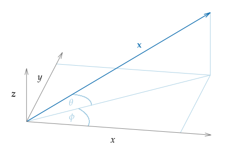
Fig. 2.1 Coordinate system used in this document. The vector \(x\) can also be described by its length, its azimuth angle \(\phi\), and its elevation \(\theta\).

2.2. Fourier transformation

Let \(s\) be an absolute integrable function, \(t,\w\) real numbers, then the temporal Fourier transform is defined after [Bra00] as

(2.1)\[S(\w) = \mathcal{F}\left\{s(t)\right\} = \int^{\infty}_{-\infty} s(t) \e{-\i\w t} \d t.\]

In the same way the inverse temporal Fourier transform is defined as

(2.2)\[s(t) = \mathcal{F}^{-1}\left\{S(\w)\right\} = \frac{1}{2\pi} \int^{\infty}_{-\infty} S(\w) \e{\i\w t} \d\w.\]